|
|
DISROC Examples |
|
| DISROC 5 - Example: |
Other Examples |
Fracture zone around tunnels
As it is well known, shear softening can lead to strain localization on shear bands which can represent mode II fractures. This example illustrates Disroc's ability to simulate this phenomenon. The model ANELVIP (31430) of the Disroc Materials Catalog covers elastoplastic materials with softening plasticity. The cohesion, friction angle and tensile strength decrease with plastic deformation.
|
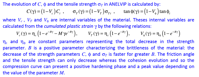
The following diagram shows the stress-strain curve of the material under uniaxial compressive load. A softening behavior is observed, with or without a positive hardening phase before the peak stress, and with different softening rates (brittleness) and different residual stresses, for different values of the constitutive parameters.
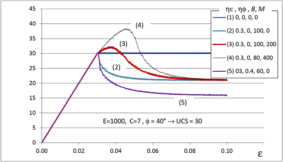 Fig.1: Softening plasticity in ANELVIP
|
Now, consider the excavation of a tunnel in quasi-brittle rock represented by the ANELVIP model with softening. The mesh and the boundary conditions used in Disroc to simulate this excavation problem are shown in the following figures.
 Fig.2a: Mesh and boundary conditions
|
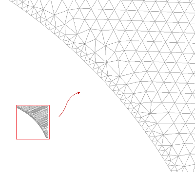
Fig.2b: Mesh zoom near the tunnel wall |
The excavation of the tunnel is modeled by controlling the boundary forces on the tunnel wall and decreasing them from
their initial values, corresponding to the in situ stresses, to zero. This process is described by the
parameter λ varying from λ =0 at the initial state of in situ stresses
to λ =1 for the totally deconfined tunnel.
The in situ stresses considered here are σH = 16 MPa and σV = 12 MPa.
The rock strength is given by the Mohr-Coulomb criterion with cohesion C=7.2 MPa and φ=12°.
The softening behavior leads to a residual cohesion of 0.3*C=2.16 MPa and a residual friction
angle of 0.2*φ=2.4°.
The following figures show the shear fractures developed around the tunnel
by this excavation action for different values of the deconfinig parameter λ.
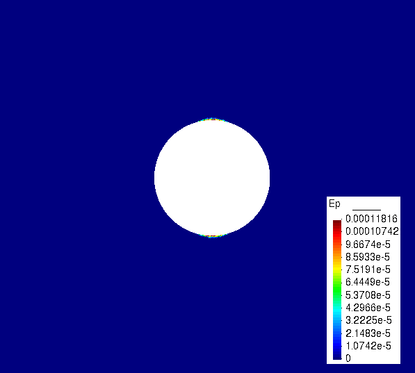 Figure 3.a: Shear fractures for λ=0.5
|
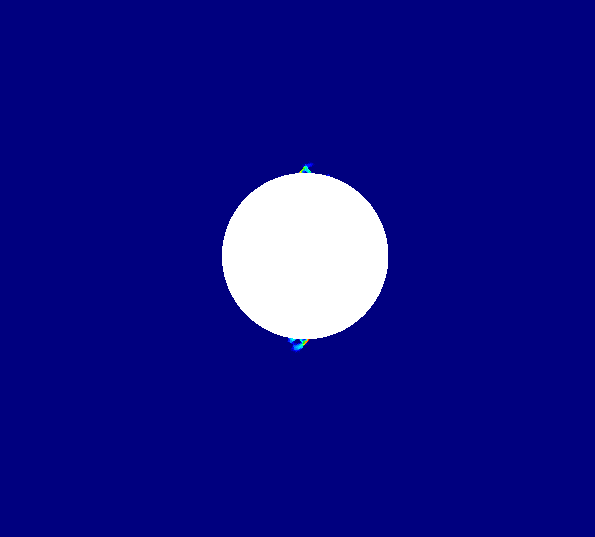 Figure 3.b: Shear fractures for λ=0.6
|
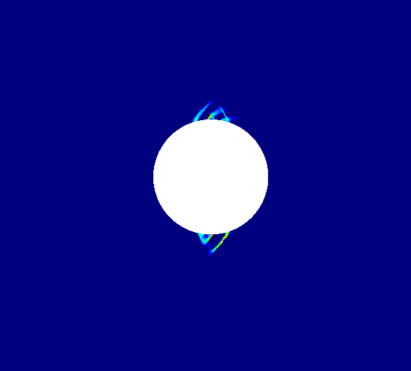 Figure 3.c: Shear fractures for λ=0.7
|
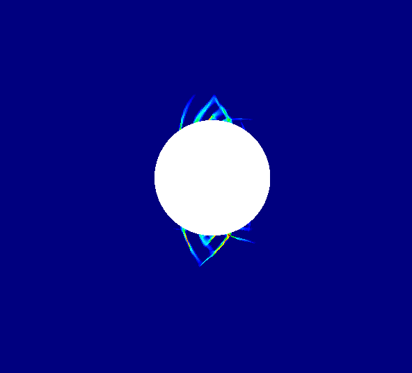 Figure 3.d: Shear fractures for λ=0.8
|
 Figure 3.e: Shear fractures for λ=0.9
|
 Figure 3.f: Shear fractures for λ=1.0
|
The state of the vertical stress σyy and vertical displacement uy at the final stage of excavation are given below.
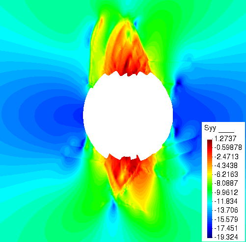 Figure 4.a: Contour of σyy (MPa) after excavation
|
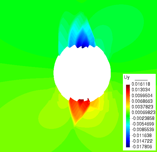 Figure 4.b: Contour of vertical displacement (m) after excavation
|
The deformed shape of the fractured excavation zone with shear bandes representing the shear fractures is given in the following figure.
Click on the figure for video animation
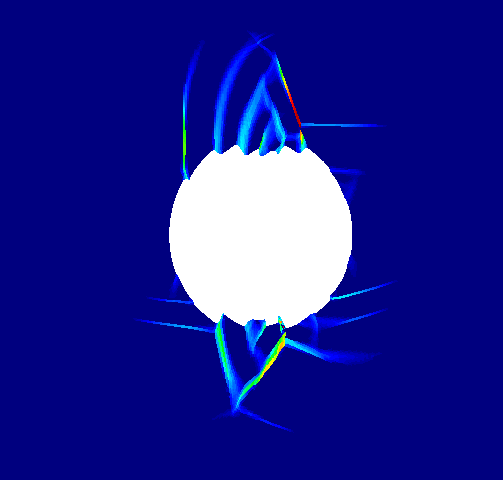
Figure 5: Shear fractures around the tunnel in deformed geometry after excavation |